How to create an Inventory Management System [using Excel] in 2021

Hello and welcome to the Mr Spreadsheet YouTube channel .

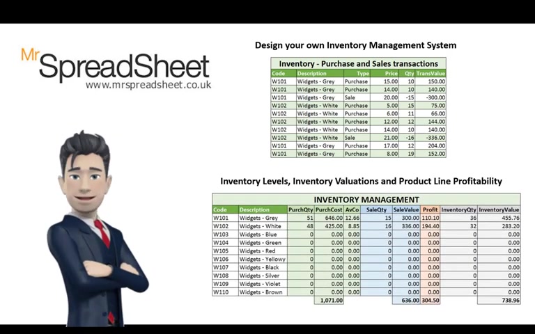
If you would like to create and design your own inventory management system using Excel spreadsheets , then this short tutorial will show you how the inventory management spreadsheet will record inventory transactions and will monitor inventory levels , inventory valuations and product line profitability .

The final template is both easy to use and to understand .

The inventory management spreadsheet will use many of Excel's functions and commands , including the use of dropdown boxes to select data .

We employ the sum if command and retrieve data using the V look up function .

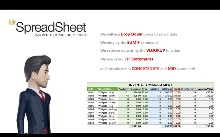
We also use if commands to isolate data and introduce the concatenate and the mid commands to perform advanced data selection routines .

As usual , I will show you how to obtain a copy of the completed template later on in this video .

And if you need any help on the Excel functions that I've used , then please do leave me a comment below .

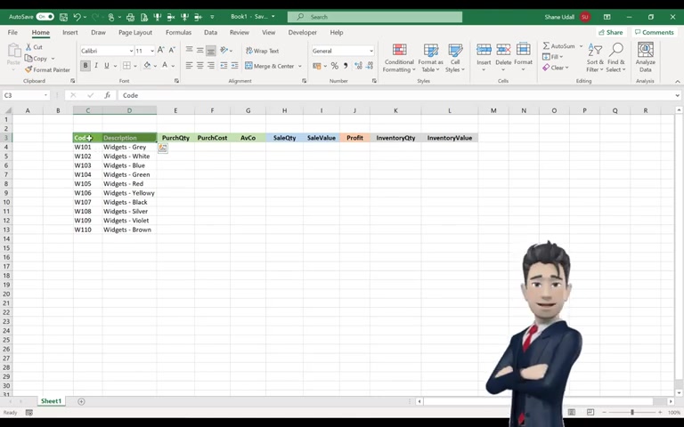
I hope you enjoy watching open up a new workbook and we will start our inventory management system by entering our 1st 10 products , Select Cell C three and enter code and in D three enter description in cells .

C four through to D 13 .

Copy in my product codes and descriptions .

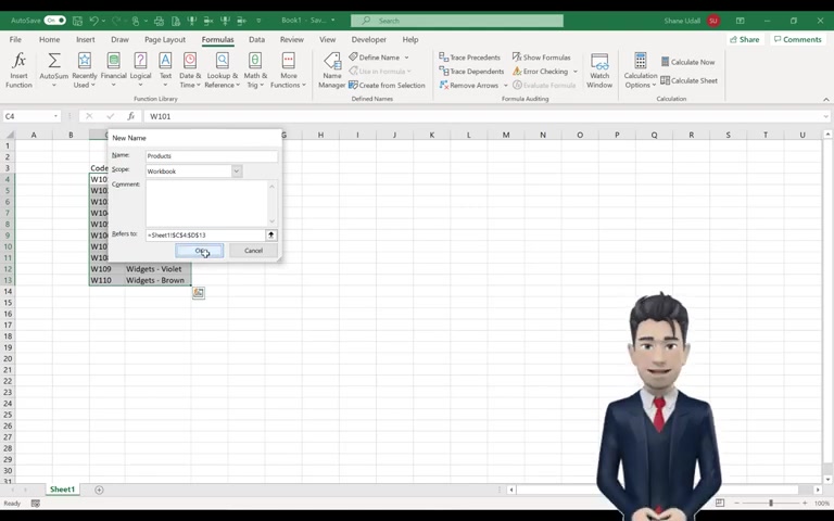
Alternatively , enter data more suited to your needs now Highlight the Range C four through to D 13 and from the Formulas Ribbon .

Select the define name tool and enter the name products and then click OK .

Our inventory management system needs to record details of inventory purchases and the cost of those purchases , so let's expand the table to accommodate these in cell E three .

Enter purchase quantity in F three .

It's purchase cost and in G three , we need the average cost .

Now we need to include details of our sales quantities and sales values , so enter cells quantity in cell H three and cells value in i three .

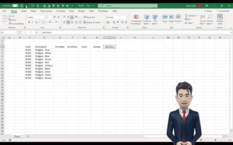
We would also like to calculate our profits for each inventory item , so enter profit in sell J three .

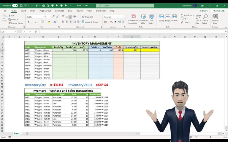
Our final two columns in this table will record the running or cumulative inventory quantities and inventory valuations for each product line .

OK , now that we have our inventory management table created , let's apply some formatting and give the table a heading .

Select the range C three through two D three and apply a background colour of green .

Select the range E three through to G three and apply a background colour of mid green .

Select the range H three through to I three and colour this mid blue J three is coloured mid orange and K three through two .

L three is coloured mid grey .

Now make bold the entire range from C three through to L three and change the font colour of C three through to D three to white .

Highlight the range C three through to L three and from the home ribbon , Select the Borders tool and apply all borders .

Highlight the range C two through to L two and use the merge and centre tool and enter inventory management as the heading .

Increase the font size and apply a background colour of light green .

Highlight the range E four through to G 13 and apply a background colour of light green .

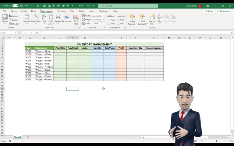
The range H four through to I 13 becomes light blue J four through to J 13 is light orange and K .

Four .

Through two , L , 13 becomes light grey and finally , from the page layout ribbon uncheck the View Grid Lines box to give our worksheet a crisp and clear background .

Now that we have defined our inventory management table , we can now create a new table to record our inventory purchases and our inventory sales .

We will create this inventory movements table in the next session .

We will create our inventory movements table by selecting cell C 18 and entering in the name code .

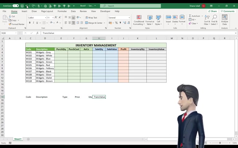
D 18 becomes description .

E 18 is type .

F-18 is price , G 18 becomes quantity and H 18 is the transaction value .

Highlight the range C 18 through to H 18 and apply a background colour of green and a font colour of white and then make bold .

Select the range C 18 through to H 28 and from the home ribbon , Select the Borders tool and apply all borders .

Now let's give this table a title .

Highlight the range C 17 through to H 17 and merge and centre these cells and then enter the title as shown .

Increase the font size and then make bold .

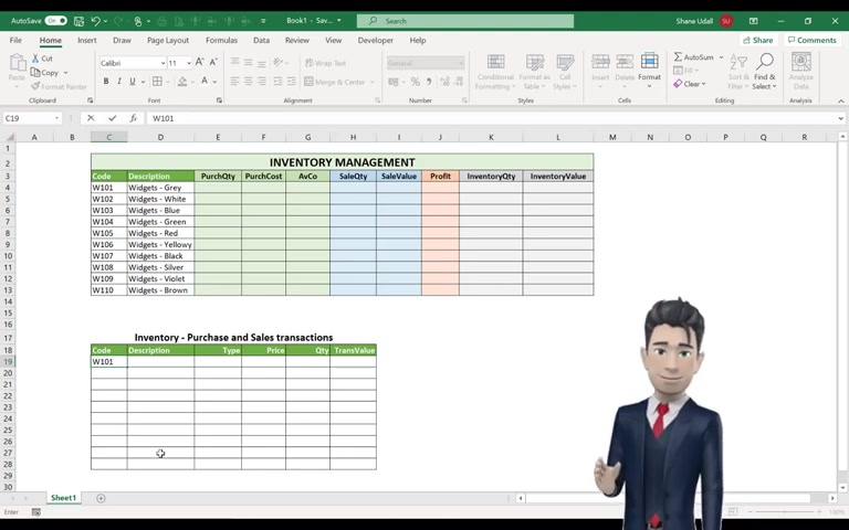
Let's enter our first inventory transaction .

Enter the product code of W 101 in cell , C 19 .

We would like the description in cell D 19 to populate automatically .

We can do this by using XL's V look up function .

You will recall that earlier in this video we gave the range C four through two .

D 13 a name .

We call this range products and we will now use this range to help us with our V Look up command .

So with D 19 selected type in the formula equals V .

Look up .

Open brackets point to cell C 19 comma Enter the word products comma , then a two a comma , the word false and now close the brackets .

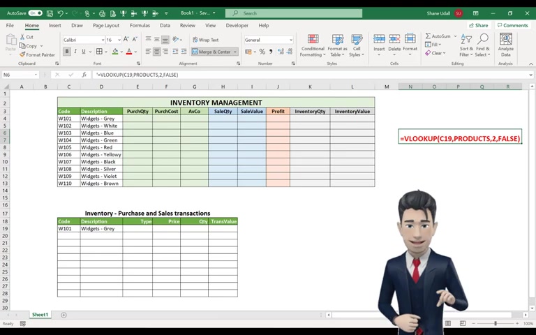
The correct description of widgets .

Grey is retrieved from the second column of the product's table .

Navigate to Cell E 19 .

We want the value in this sale to be either purchase or sale .

We can use Excel's data validation tool to achieve this with E 19 still active .

Select the data ribbon and then pick up the data validation tool from the dialogue box that opens .

Choose list from the allow field and in the source field .

Type in purchase , followed by a comma , followed by sale with no spaces and now click OK cell .

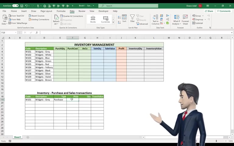
E 19 now contains a drop down box from which you can choose which type of transaction this is Please select purchase .

We can now complete our first transaction long enter price of 15 and a quantity of 10 in cells F 19 and G 19 .

Our transaction value is simply F 19 multiplied by G 19 .

So enter this formula into cell age 19 .

Now let's copy our formula down to the end of the inventory movements table .

Highlight the range D 19 through to E 19 and now copy and drag down these formula to the end of the table in Row 28 .

Similarly , highlight cell H 19 and copy and drag this down to H 28 .

That's great .

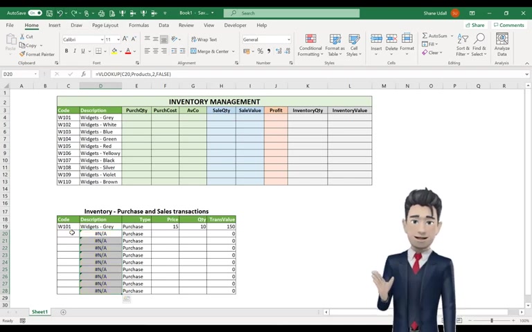
All the formula in the in imagery movements table have now been entered .

However , all the description lines apart from D 19 are showing the N a error message .

This is simply because the Description field is totally dependent on there being a valid code in the code field as all of these are currently blank , Then the N error message is returned .

We can correct this by using a simple if statement in front of our V .

Look up command in the description fields .

This if statement will examine the contents of the code column , and if the column entry is blank , then the description will also return a blank Select cell , D 19 and in the command line , place your cursor after the equal sign and before the VA V .

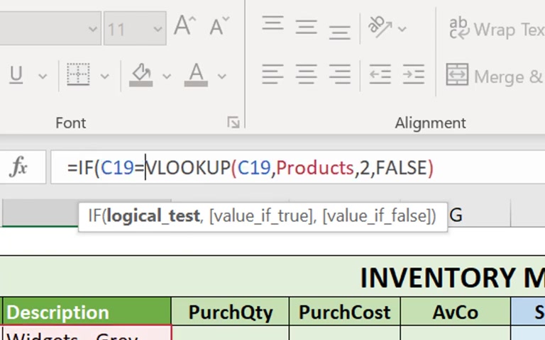
Look up and then enter the following if open brackets .

Then 0.2 Cell C , 19 equals inverted comma , inverted comma , followed by a comma , inverted comma , inverted comma again followed by a comma and then navigate to the end of the formula and add in a final closing brackets .

Now with C 19 still highlighted copy and drag down the new formula to D 28 .

Hopefully , the error message now disappears .

Finally , in this section delete the contents of E , 20 to E 28 .

The narrative hopefully disappears , but the drop down boxes will still remain .

Now select the Ranges F 19 to F 28 and H 19 to H 28 and format the number to two decimal places .

In the next section , we will begin to update the inventory management table with the data entered in the inventory movements table .

In order to create our formula for the inventory management table , we need some transaction data in the inventory movement schedule .

So please pause the video whilst you enter the additional nine lines of data in the movement table , noting that sales quantities are recorded as negative values .

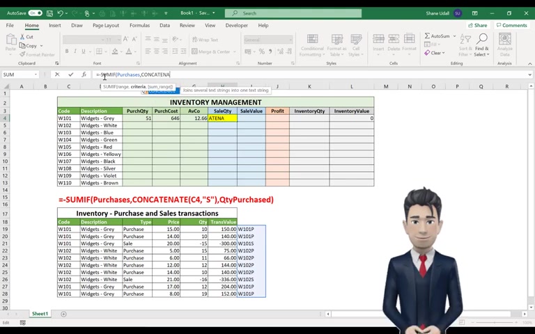
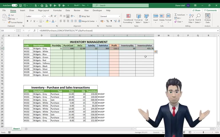
Now select cell E four and enter in .

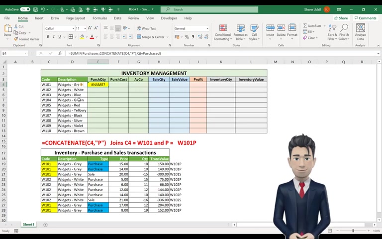
The following formula equals some if open brackets the word purchases followed by a comma and then the command concatenate open brackets 0.2 cell C four enter a comma .

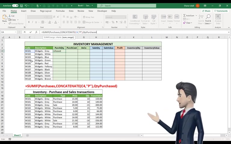
Then it's inverted comma , followed by a P , followed by inverted comma Close the brackets , then another comma , then the word quantity purchased .

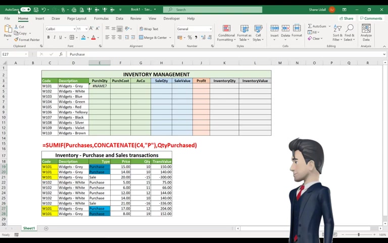
And now close the brackets Ignore the name error message that this formula returns .

And now I will explain all the elements of this formula and how it helps us to accurately complete our purchase quantity values .

Our first formula in the inventory management table needs to collect all instances where there is a purchase of product W 101 in the transaction table .

Now we can see that there are five transactions for product W 101 Now .

Of these five transactions , four are purchases and one is a sale .

Our purchase quantity formula only requires that we select the four purchases and that we ignore any sales transactions .

Our formula therefore needs to select all instances where W 101 is the product and the transaction type is purchase .

We can achieve this by using a sum if command which we have already entered in cell E four .

But first of all , we need some way to identify the instances of purchases of product .

W 101 navigate To sell i 19 , we're going to create a formula that specifically identifies and matches products with their transaction type .

So enter the following formula into cell by 19 equals concatenate Open brackets point to cell C 19 Enter a comma and then the command mid open brackets point to E .

19 .

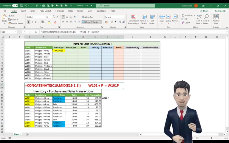
Enter a comma , then a one , then a comma and then another one and then finally two closing brackets .

The Concatenate Command says Join the following criteria together to form a single string .

C 19 refers to W 101 and the command of mid open bracket E 19 comma , one comma one closed brackets says examine the contents of cell E 19 , which in our case , is equal to the word purchase and from the word purchase return the first character which equals P concatenate or join these two together and you get the string W 101 P .

We now have correctly analysed the contents of the two cells and created a unique code for it which will help us in the sum if command .

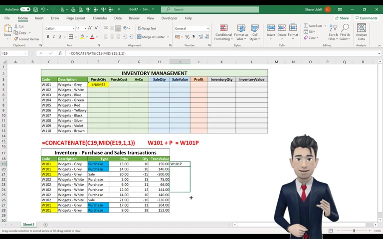
Now let's copy this formula down from I 19 all the way down to the end of the table in I 28 .

Each line picks up the relevant product code and then adds either a P or an S to it .

This now makes our use of the sum if command a lot easier , as we now have a unique criteria range from which to aggregate our purchase quantity data .

Our selection range of I 19 to I 28 needs to be given a name so that the sum if command can pick up the correct values .

So highlight I 19 through to I 28 and give this a name by selecting the defined name command from the formula's ribbon .

Enter the name purchases and click OK , the second element of the sum .

If command in cell E four of the inventory management table is the criteria W 101 in cell C four .

But we need this W 101 to match the corresponding value from our purchases in the range I 19 to I 28 .

All of these will return the extended values of W 101 plus either an S or a P .

So returning to our formula in cell E four , we need to join together or concatenate the value in C four , which is W 101 and the letter P Finally in the Summit Command , we need to identify and name the quantity purchase range .

This is in fact , the range G 19 through to G 28 .

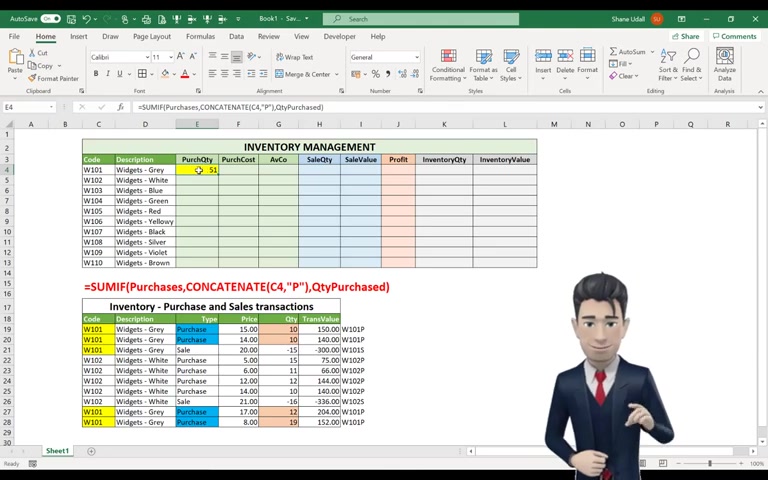
So highlight this range and from the formulas ribbon select the defined a tool and enter quantity purchased with no spaces in the name field .

And now click OK , hopefully your sum If command is now showing a value of 51 which is the aggregate value of all the items shown in the orange cells in the inventory movements table , please don't worry .

If you do not get the entire process right on your first attempt , the process is quite advanced .

But once mastered , it will prove an invaluable technique going forward .

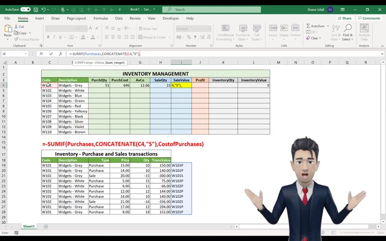
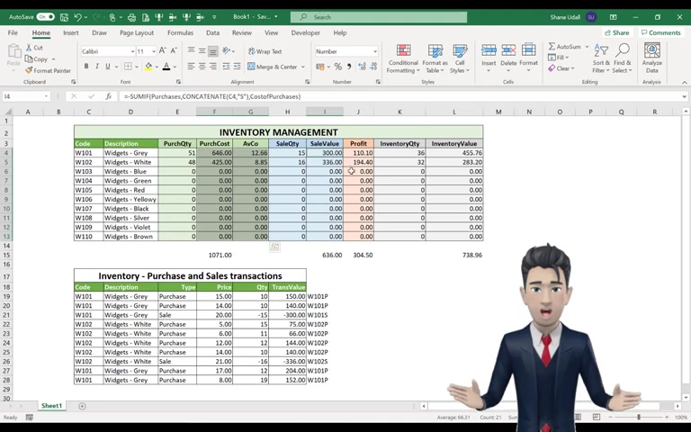
Let's use a similar formula to calculate the cost of all of our purchases of product .

W 101 .

We will use the sum if command again and pick up all the relevant values in the inventory movements table .

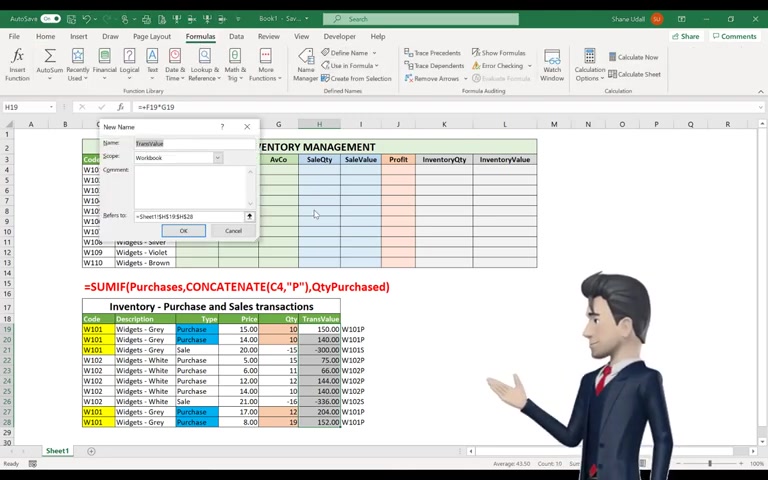
But first , let's name the transaction value range , so highlight cells H 19 to 28 and select the formulas ribbon from here .

Choose the defined name command and use the name of cost of purchases without any spaces and click OK , navigate back to cell F four and enter in .

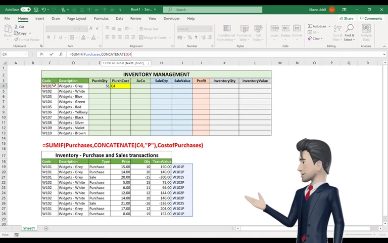
The following formula equals some if open brackets the word purchases , then a comma , then the command concatenate open brackets 0.2 C four inverted comma , followed by a P and then another inverted comma and close the bracket , then another comma and then the word cost of purchases and close the bracket Cell F four should populate with 646.00 which is the aggregate value of all purchases of product .

W 101 .

The average unit cost of purchases of product W 101 is simply F four divided by E four .

So enter this formula into cell G four .

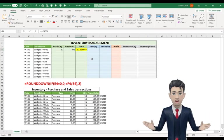
This returns a rather ugly looking value to six decimal places , and we also know that if there was no value in the purchase quantity field , this formula will return a divided by zero error .

So let's correct both of these .

Firstly , change the formula in E four to read If open brackets E four equals zero comma , then a zero , then a comma and then F four , divided by E four and close the brackets .

Now , if we have a nil value in E four , the formula does not return an error message .

Now let's add the round down command such that our previous formula in G four is nested with round down , set to two decimal places .

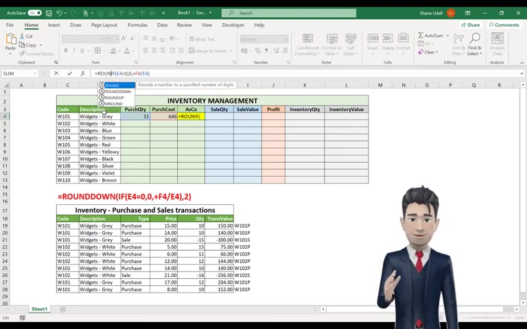
The entire formula now reads , equals round down open brackets .

If open brackets point to E , four equals zero comma , then a zero , then another comma and then plus F four divided by E four and close the brackets and then finally a comma and then two and close the final bracket .

Our sale quantity uses exactly the same formula as our purchase quantity formula , the only difference being that instead of using a P for purchase , we use an S for sale , so enter the formula as follows equals minus some .

If open brackets purchases comma concatenate open brackets 0.2 C four comma , then inverted comma , then S , then inverted comma and close the brackets , then a comma and then quantity purchased and close the brackets .

The table returns the aggregate sales quantity extracted from the inventory movement schedule .

We can do exactly the same for our cell value .

The formula becomes equals minus some if open brackets purchases comma concatenate open brackets 0.2 cell C four comma inverted comma S inverted comma .

Close the brackets comma and then cost of purchases and close the brackets .

Hopefully , the formula will return the value of 300 which is the aggregate value taken from the inventory movement schedule .

The aggregate profit formula in cell J four is simply the total sales value in I form less the sales quantity multiplied by the average cost .

So in J four enter equals plus I four minus open brackets point to G four times point to H four and close the brackets .

The correct profit figure of 110.10 is returned .

A cumulative inventory quantity is the total purchase quantity less the total sales quantity so enter the formula equals plus four minus H four into cell K form and our cumulative inventory valuation is simply the inventory quantity in cell K four multiplied by the unit average cost in G four .

So enter the formula equals K four times G four into cell L four .

Hopefully , the values of 36 and 455.76 are returned .

Now that we have entered all on formula for the first product , W 101 , we can now apply these formula to the remaining nine products , so highlight the range E four through two L four and copy and drag the contents down to row 13 .

That's great .

It all seems to be working fine .

Let's complete our work by adding a few totals , applying various cell formats and hiding or deleting unwanted data or values .

Let's have some totals for total purchase cost , total sales value , total profit and total inventory valuation .

Select cell F-15 and then simply double click the auto su tool .

Select cells by 15 J 15 and L 15 and repeat the auto sum command now highlight the ranges F four through two , G 13 i 432 , J 13 and L four through to L 13 .

And then right , click your mouse .

Select the format cells option and then the numbers tab and then number .

And then set these to two decimal places with the 1000 comma separator checked .

Finally highlight the range I 19 through to I 28 and change the font colour to white such that these values are now hidden .

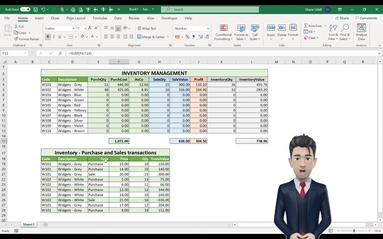
Use the format painter tool to change the background colours of our total fields and then make these bold and finally apply some alternate line formatting to our inventory movements table and that completes our design work .

We now have a fully functioning inventory management system which we hope will be of use to both you and your business .

We do hope that you enjoyed our inventory management spreadsheet tutorial and that there was lots of content that you found both useful and informative .

Now , if you would like us to send you a copy of the completed template , then please give this video a big thumbs up and subscribe to our YouTube channel .

Alternatively , please visit one of our channels on either Facebook , Instagram or Twitter .

Now , if you are a small business and you want to keep your business accounts records in Excel , then why not watch our accounting spreadsheet tutorial ?

Alternatively , why not take a look at our how to keep inventory in Excel video ?

This popular tutorial shows you how to create a more basic inventory management tool .